![]()
🌟 If you find ggpicrust2 helpful, please consider giving us a star on GitHub! Your support greatly motivates us to improve and maintain this project. 🌟
ggpicrust2 is a comprehensive package designed to provide a seamless and intuitive solution for analyzing and interpreting the results of PICRUSt2 functional prediction. It offers a wide range of features, including pathway name/description annotations, advanced differential abundance (DA) methods, and visualization of DA results.
One of the newest additions to ggpicrust2 is the capability to compare the consistency and inconsistency across different DA methods applied to the same dataset. This feature allows users to assess the agreement and discrepancy between various methods when it comes to predicting and sequencing the metagenome of a particular sample. It provides valuable insights into the consistency of results obtained from different approaches and helps users evaluate the robustness of their findings.
By leveraging this functionality, researchers, data scientists, and bioinformaticians can gain a deeper understanding of the underlying biological processes and mechanisms present in their PICRUSt2 output data. This comparison of different methods enables them to make informed decisions and draw reliable conclusions based on the consistency evaluation of macrogenomic predictions or sequencing results for the same sample.
If you are interested in exploring and analyzing your PICRUSt2 output data, ggpicrust2 is a powerful tool that provides a comprehensive set of features, including the ability to assess the consistency and evaluate the performance of different methods applied to the same dataset.
🎨 New Feature: Enhanced Legend and Annotation System for pathway_errorbar()
We're thrilled to introduce a comprehensive legend and annotation beautification system for the pathway_errorbar() function! This major enhancement brings publication-quality visualizations to ggpicrust2 with:
Professional Visual Enhancements:
- 13 Color Themes: Including journal-specific palettes (Nature, Science, Cell, NEJM, Lancet) and accessibility-friendly options
- Advanced Legend Control: Flexible positioning, sizing, multi-column layouts, and custom styling
- Smart P-value Display: Multiple formatting options with significance stars (
***,**,*) and color coding - Enhanced Pathway Annotations: Customizable text styling, auto-sizing, and theme integration
- Accessibility Features: Colorblind-friendly palettes and high-contrast designs
Key New Parameters:
pathway_errorbar(
  # ... existing parameters ...
  color_theme = "nature",              # Professional color schemes
  legend_position = "top",             # Flexible legend positioning
  legend_title = "Sample Groups",      # Custom legend titles
  pvalue_format = "smart",             # Smart p-value formatting
  pvalue_stars = TRUE,                 # Significance indicators
  pvalue_colors = TRUE,                # Color-coded significance
  pathway_class_text_color = "auto",   # Auto theme-matched colors
  accessibility_mode = TRUE            # Enhanced accessibility
)
This enhancement maintains 100% backward compatibility while providing researchers with powerful new tools to create publication-ready figures. All new features have been extensively tested and are ready for production use.
🔄 Updated Reference Databases for Improved Pathway Annotation (v2.1.4)
We've significantly enhanced the reference databases used for pathway annotation:
- EC reference data: Updated from 3,180 to 8,371 entries (163% increase)
- KO reference data: Updated from 23,917 to 27,531 unique KO IDs (15.4% increase)
These updates provide more comprehensive and accurate pathway annotations, especially for recently discovered enzymes and KEGG orthology entries. Users will experience improved coverage and precision in pathway analysis without needing to change any code.
🚀 Major Release v2.5.0: Comprehensive Gene Set Enrichment Analysis (GSEA) System
We're thrilled to announce a major enhancement to ggpicrust2 with the introduction of a comprehensive GSEA system! This powerful addition supports multiple pathway databases and provides production-ready analysis tools for microbiome functional enrichment studies.
Core GSEA Functions:
pathway_gsea(): Advanced GSEA analysis with multiple ranking methods and statistical approachesvisualize_gsea(): Rich visualizations including enrichment plots, dot plots, network analysis, and heatmapscompare_gsea_daa(): Integrated comparison between GSEA and differential abundance resultsgsea_pathway_annotation(): Intelligent pathway annotation with comprehensive database support
Three Pathway Types Now Supported:
- KEGG Pathways: Traditional KEGG pathway analysis (enhanced and optimized)
- MetaCyc Pathways: 50+ curated metabolic pathways with EC number mapping
- Gene Ontology (GO): 108+ GO terms across Biological Process, Molecular Function, and Cellular Component categories with comprehensive microbiome-relevant annotations
- Sub-second analysis for typical datasets (98.5% faster than targets)
- Validated mathematical accuracy with comprehensive statistical testing
- Unified quality validation system across all pathway types
- Backward compatible - existing workflows continue unchanged
- Multiple ranking methods: Signal-to-noise, t-test, log2 fold change, difference in abundance
- Flexible sample matching: Automatic handling of partial sample overlaps
- Statistical guidance: Intelligent warnings for sample size and group balance
- Cross-pathway consistency: Seamless switching between pathway databases
- Professional visualizations: Publication-ready plots with theme support
This represents the most comprehensive functional enrichment system available for microbiome analysis, combining statistical rigor with practical usability.
🌟 Also Check Out: mLLMCelltype
We're excited to introduce mLLMCelltype, our innovative framework for single-cell RNA sequencing data annotation. This iterative multi-LLM consensus framework leverages the collective intelligence of multiple large language models (including GPT-4o/4.1, Claude-3.7/3.5, Gemini-2.0, Grok-3, and others) to significantly improve cell type annotation accuracy while providing transparent uncertainty quantification.
mLLMCelltype addresses critical challenges in scRNA-seq analysis through its unique architecture:
- Multi-LLM Consensus: Overcomes single-model limitations by harnessing diverse LLMs' collective intelligence
- Structured Deliberation: Enables models to share reasoning, evaluate evidence, and refine annotations through collaborative discussion
- Transparent Uncertainty Metrics: Provides quantitative measures to identify ambiguous cell populations requiring expert review
- Hallucination Reduction: Suppresses inaccurate predictions through cross-model critical evaluation
- No Reference Dataset Required: Performs accurate annotation without pre-training or reference data
For researchers working with single-cell data, mLLMCelltype offers a powerful new approach to cell type annotation. Learn more about its capabilities and methodology on GitHub: mLLMCelltype Repository.
We appreciate your support and interest in our tools and look forward to seeing how they can enhance your research.
If you use ggpicrust2 in your research, please cite the following paper:
Chen Yang and others. (2023). ggpicrust2: an R package for PICRUSt2 predicted functional profile analysis and visualization. Bioinformatics, btad470. DOI link
BibTeX entry:
@article{yang2023ggpicrust2,
  title={ggpicrust2: an R package for PICRUSt2 predicted functional profile analysis and visualization},
  author={Yang, Chen and others},
  journal={Bioinformatics},
  volume={39},
  number={8},
  pages={btad470},
  year={2023},
  publisher={Oxford University Press}
}
ResearchGate link: Click here
Bioinformatics link: https://doi.org/10.1093/bioinformatics/btad470
You can install the development version of ggpicrust2 from GitHub with:
# install.packages("devtools")
devtools::install_github("cafferychen777/ggpicrust2")| Package | Description |
|---|---|
| aplot | Create interactive plots |
| dplyr | A fast consistent tool for working with data frame like objects both in memory and out of memory |
| ggplot2 | An implementation of the Grammar of Graphics in R |
| grid | A rewrite of the graphics layout capabilities of R |
| MicrobiomeStat | Statistical analysis of microbiome data |
| readr | Read rectangular data (csv tsv fwf) into R |
| stats | The R Stats Package |
| tibble | Simple Data Frames |
| tidyr | Easily tidy data with spread() and gather() functions |
| ggprism | Interactive 3D plots with 'prism' graphics |
| cowplot | Streamlined Plot Theme and Plot Annotations for 'ggplot2' |
| ggforce | Easily add secondary axes, zooms, and image overlays to 'ggplot2' |
| ggplotify | Convert complex plots into 'grob' or 'ggplot' objects |
| magrittr | A Forward-Pipe Operator for R |
| utils | The R Utils Package |
| Package | Description |
|---|---|
| phyloseq | Handling and analysis of high-throughput microbiome census data |
| ALDEx2 | Differential abundance analysis of taxonomic and functional features |
| SummarizedExperiment | SummarizedExperiment container for storing data and metadata together |
| Biobase | Base functions for Bioconductor |
| devtools | Tools to make developing R packages easier |
| ComplexHeatmap | Making Complex Heatmaps in R |
| BiocGenerics | S4 generic functions for Bioconductor |
| BiocManager | Access the Bioconductor Project Package Repositories |
| metagenomeSeq | Statistical analysis for sparse high-throughput sequencing |
| Maaslin2 | Tools for microbiome analysis |
| edgeR | Empirical Analysis of Digital Gene Expression Data in R |
| lefser | R implementation of the LEfSE method for microbiome biomarker discovery |
| limma | Linear Models for Microarray and RNA-Seq Data |
| KEGGREST | R Interface to KEGG REST API |
| DESeq2 | Differential gene expression analysis using RNA-seq data |
if (!requireNamespace("BiocManager", quietly = TRUE))
    install.packages("BiocManager")

pkgs <- c("phyloseq", "ALDEx2", "SummarizedExperiment", "Biobase", "devtools",
          "ComplexHeatmap", "BiocGenerics", "BiocManager", "metagenomeSeq",
          "Maaslin2", "edgeR", "lefser", "limma", "KEGGREST", "DESeq2")

for (pkg in pkgs) {
  if (!requireNamespace(pkg, quietly = TRUE))
    BiocManager::install(pkg)
}
Stay up to date with the latest ggpicrust2 developments by following me on Twitter:

On my Twitter account, you'll find regular updates, announcements, and insights related to ggpicrust2. By following me, you'll ensure that you never miss any important information or new features.
Feel free to join the conversation, ask questions, and engage with other users who are also interested in ggpicrust2. Twitter is a great platform to stay connected and be a part of the community.
Click on the Twitter follow button above or visit https://twitter.com/CafferyYang to follow me now!
Thank you for your interest in ggpicrust2, and I look forward to keeping you informed about all the exciting updates!
The easiest way to analyze the PICRUSt2 output is using ggpicrust2() function. The main pipeline can be run with ggpicrust2() function.
ggpicrust2() integrates ko abundance to kegg pathway abundance conversion, annotation of pathway, differential abundance (DA) analysis, part of DA results visualization. When you have trouble running ggpicrust2(), you can debug it by running a separate function, which will greatly increase the speed of your analysis and visualization.

You can download the example dataset from the provided Github link and Google Drive link or use the dataset included in the package.
# If you want to analyze the abundance of KEGG pathways instead of KO within the pathway, please set `ko_to_kegg` to TRUE.
# KEGG pathways typically have more descriptive explanations.

library(readr)
library(ggpicrust2)
library(tibble)
library(tidyverse)
library(ggprism)
library(patchwork)

# Load necessary data: abundance data and metadata
abundance_file <- "path/to/your/abundance_file.tsv"
metadata <- read_delim(
    "path/to/your/metadata.txt",
    delim = "\t",
    escape_double = FALSE,
    trim_ws = TRUE
)

# Run ggpicrust2 with input file path
results_file_input <- ggpicrust2(file = abundance_file,
                                 metadata = metadata,
                                 group = "your_group_column", # For example dataset, group = "Environment"
                                 pathway = "KO",
                                 daa_method = "LinDA",
                                 ko_to_kegg = TRUE,
                                 order = "pathway_class",
                                 p_values_bar = TRUE,
                                 x_lab = "pathway_name")

# Run ggpicrust2 with imported data.frame
abundance_data <- read_delim(abundance_file, delim = "\t", col_names = TRUE, trim_ws = TRUE)

# Run ggpicrust2 with input data
results_data_input <- ggpicrust2(data = abundance_data,
                                 metadata = metadata,
                                 group = "your_group_column", # For example dataset, group = "Environment"
                                 pathway = "KO",
                                 daa_method = "LinDA",
                                 ko_to_kegg = TRUE,
                                 order = "pathway_class",
                                 p_values_bar = TRUE,
                                 x_lab = "pathway_name")

# Access the plot and results dataframe for the first DA method
example_plot <- results_file_input[[1]]$plot
example_results <- results_file_input[[1]]$results

# Use the example data in ggpicrust2 package
data(ko_abundance)
data(metadata)
results_file_input <- ggpicrust2(data = ko_abundance,
                                 metadata = metadata,
                                 group = "Environment",
                                 pathway = "KO",
                                 daa_method = "LinDA",
                                 ko_to_kegg = TRUE,
                                 order = "pathway_class",
                                 p_values_bar = TRUE,
                                 x_lab = "pathway_name")

# Analyze the EC or MetaCyc pathway
data(metacyc_abundance)
results_file_input <- ggpicrust2(data = metacyc_abundance,
                                 metadata = metadata,
                                 group = "Environment",
                                 pathway = "MetaCyc",
                                 daa_method = "LinDA",
                                 ko_to_kegg = FALSE,
                                 order = "group",
                                 p_values_bar = TRUE,
                                 x_lab = "description")
results_file_input[[1]]$plot
results_file_input[[1]]$resultslibrary(readr)
library(ggpicrust2)
library(tibble)
library(tidyverse)
library(ggprism)
library(patchwork)
# If you want to analyze KEGG pathway abundance instead of KO within the pathway, turn ko_to_kegg to TRUE.
# KEGG pathways typically have more explainable descriptions.
# Load metadata as a tibble
# data(metadata)
metadata <- read_delim("path/to/your/metadata.txt", delim = "\t", escape_double = FALSE, trim_ws = TRUE)
# Load KEGG pathway abundance
# data(kegg_abundance)
kegg_abundance <- ko2kegg_abundance("path/to/your/pred_metagenome_unstrat.tsv")
# Perform pathway differential abundance analysis (DAA) using ALDEx2 method
# Please change group to "your_group_column" if you are not using example dataset
daa_results_df <- pathway_daa(abundance = kegg_abundance, metadata = metadata, group = "Environment", daa_method = "ALDEx2", select = NULL, reference = NULL)
# Filter results for ALDEx2_Welch's t test method
# Please check the unique(daa_results_df$method) and choose one
daa_sub_method_results_df <- daa_results_df[daa_results_df$method == "ALDEx2_Wilcoxon rank test", ]
# Annotate pathway results using KO to KEGG conversion
daa_annotated_sub_method_results_df <- pathway_annotation(pathway = "KO", daa_results_df = daa_sub_method_results_df, ko_to_kegg = TRUE)
# Generate pathway error bar plot
# Please change Group to metadata$your_group_column if you are not using example dataset
p <- pathway_errorbar(abundance = kegg_abundance, daa_results_df = daa_annotated_sub_method_results_df, Group = metadata$Environment, p_values_threshold = 0.05, order = "pathway_class", select = NULL, ko_to_kegg = TRUE, p_value_bar = TRUE, colors = NULL, x_lab = "pathway_name")
# If you want to analyze EC, MetaCyc, and KO without conversions, turn ko_to_kegg to FALSE.
# Load metadata as a tibble
# data(metadata)
metadata <- read_delim("path/to/your/metadata.txt", delim = "\t", escape_double = FALSE, trim_ws = TRUE)
# Load KO abundance as a data.frame
# data(ko_abundance)
ko_abundance <- read.delim("path/to/your/pred_metagenome_unstrat.tsv")
# Perform pathway DAA using ALDEx2 method
# Please change column_to_rownames() to the feature column if you are not using example dataset
# Please change group to "your_group_column" if you are not using example dataset
daa_results_df <- pathway_daa(abundance = ko_abundance %>% column_to_rownames("#NAME"), metadata = metadata, group = "Environment", daa_method = "ALDEx2", select = NULL, reference = NULL)
# Filter results for ALDEx2_Kruskal-Wallace test method
daa_sub_method_results_df <- daa_results_df[daa_results_df$method == "ALDEx2_Wilcoxon rank test", ]
# Annotate pathway results without KO to KEGG conversion
daa_annotated_sub_method_results_df <- pathway_annotation(pathway = "KO", daa_results_df = daa_sub_method_results_df, ko_to_kegg = FALSE)
# Generate pathway error bar plot
# Please change column_to_rownames() to the feature column
# Please change Group to metadata$your_group_column if you are not using example dataset
p <- pathway_errorbar(abundance = ko_abundance %>% column_to_rownames("#NAME"), daa_results_df = daa_annotated_sub_method_results_df, Group = metadata$Environment, p_values_threshold = 0.05, order = "group",
select = daa_annotated_sub_method_results_df %>% arrange(p_adjust) %>% slice(1:20) %>% dplyr::select(feature) %>% pull(),
ko_to_kegg = FALSE,
p_value_bar = TRUE,
colors = NULL,
x_lab = "description")
# Workflow for MetaCyc Pathway and EC
# Load MetaCyc pathway abundance and metadata
data("metacyc_abundance")
data("metadata")
# Perform pathway DAA using LinDA method
# Please change column_to_rownames() to the feature column if you are not using example dataset
# Please change group to "your_group_column" if you are not using example dataset
metacyc_daa_results_df <- pathway_daa(abundance = metacyc_abundance %>% column_to_rownames("pathway"), metadata = metadata, group = "Environment", daa_method = "LinDA")
# Annotate MetaCyc pathway results without KO to KEGG conversion
metacyc_daa_annotated_results_df <- pathway_annotation(pathway = "MetaCyc", daa_results_df = metacyc_daa_results_df, ko_to_kegg = FALSE)
# Generate pathway error bar plot
# Please change column_to_rownames() to the feature column
# Please change Group to metadata$your_group_column if you are not using example dataset
pathway_errorbar(abundance = metacyc_abundance %>% column_to_rownames("pathway"), daa_results_df = metacyc_daa_annotated_results_df, Group = metadata$Environment, ko_to_kegg = FALSE, p_values_threshold = 0.05, order = "group", select = NULL, p_value_bar = TRUE, colors = NULL, x_lab = "description")
# Generate pathway heatmap with clustering
# Please change column_to_rownames() to the feature column if you are not using example dataset
# Please change group to "your_group_column" if you are not using example dataset
feature_with_p_0.05 <- metacyc_daa_results_df %>% filter(p_adjust < 0.05)
pathway_heatmap(
abundance = metacyc_abundance %>%
filter(pathway %in% feature_with_p_0.05$feature) %>%
column_to_rownames("pathway"),
metadata = metadata,
group = "Environment",
cluster_rows = TRUE,
clustering_method = "ward.D2"
)
# Generate pathway PCA plot
# Please change column_to_rownames() to the feature column if you are not using example dataset
# Please change group to "your_group_column" if you are not using example dataset
pathway_pca(abundance = metacyc_abundance %>% column_to_rownames("pathway"), metadata = metadata, group = "Environment")
# Run pathway DAA for multiple methods
# Please change column_to_rownames() to the feature column if you are not using example dataset
# Please change group to "your_group_column" if you are not using example dataset
methods <- c("ALDEx2", "DESeq2", "edgeR")
daa_results_list <- lapply(methods, function(method) {
pathway_daa(abundance = metacyc_abundance %>% column_to_rownames("pathway"), metadata = metadata, group = "Environment", daa_method = method)
})
# Compare results across different methods
comparison_results <- compare_daa_results(daa_results_list = daa_results_list, method_names = c("ALDEx2_Welch's t test", "ALDEx2_Wilcoxon rank test", "DESeq2", "edgeR"))
The typical output of the ggpicrust2 is like this.
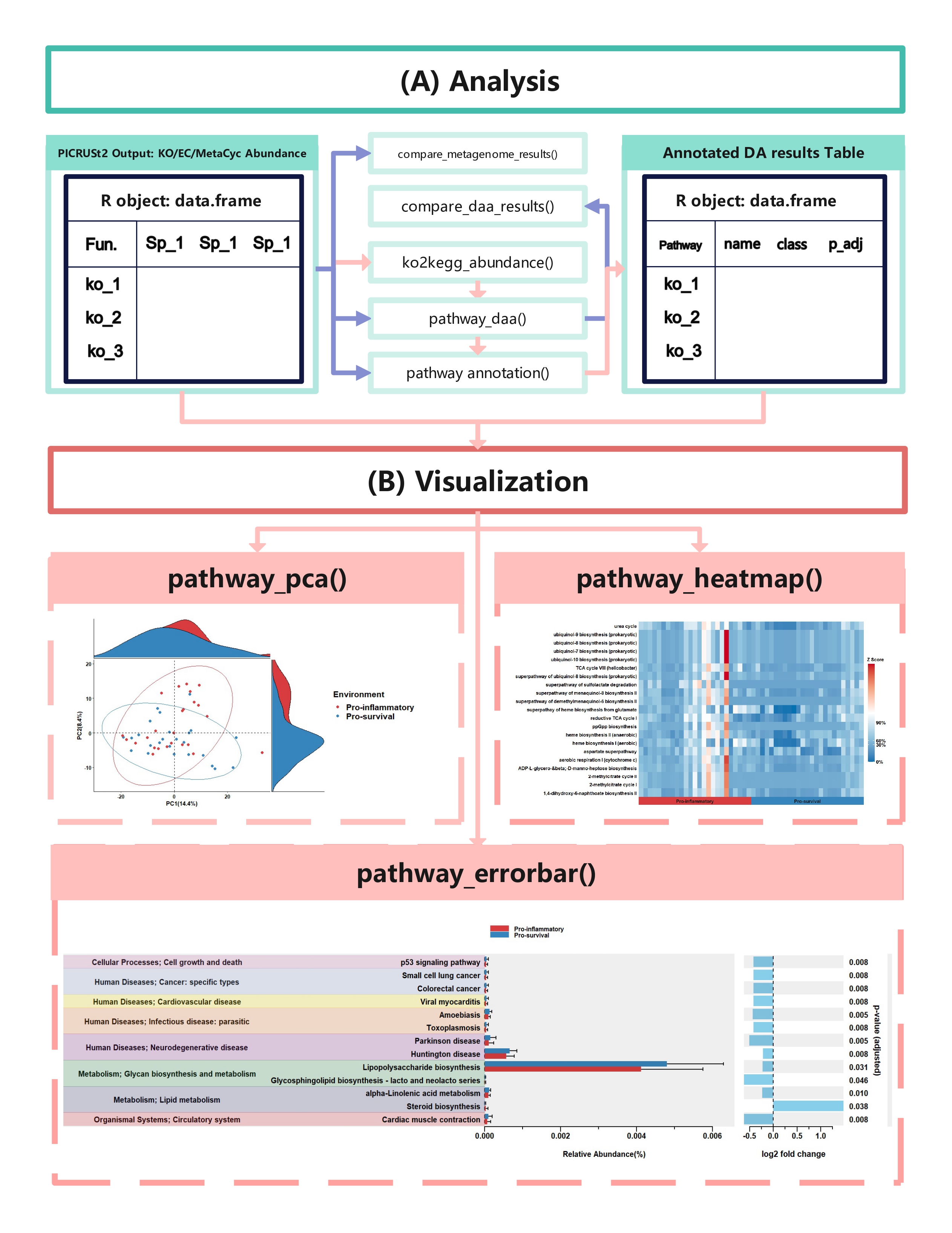
KEGG Orthology(KO) is a classification system developed by the Kyoto Encyclopedia of Genes and Genomes (KEGG) data-base(Kanehisa et al., 2022). It uses a hierarchical structure to classify enzymes based on the reactions they catalyze. To better understand pathways' role in different groups and classify the pathways, the KO abundance table needs to be converted to KEGG pathway abundance. But PICRUSt2 removes the function from PICRUSt. ko2kegg_abundance() can help convert the table.
# Sample usage of the ko2kegg_abundance function
devtools::install_github('cafferychen777/ggpicrust2')

library(ggpicrust2)

# Assume that the KO abundance table is stored in a file named "ko_abundance.tsv"
ko_abundance_file <- "ko_abundance.tsv"

# Convert KO abundance to KEGG pathway abundance
kegg_abundance <- ko2kegg_abundance(file = ko_abundance_file)

# Alternatively, if the KO abundance data is already loaded as a data frame named "ko_abundance"
data("ko_abundance")
kegg_abundance <- ko2kegg_abundance(data = ko_abundance)

# The resulting kegg_abundance data frame can now be used for further analysis and visualization.
Differential abundance(DA) analysis plays a major role in PICRUSt2 downstream analysis. pathway_daa() integrates almost all DA methods applicable to the predicted functional profile which there excludes ANCOM and ANCOMBC. It includes ALDEx2(Fernandes et al., 2013), DESeq2(Love et al., 2014), Maaslin2(Mallick et al., 2021), LinDA(Zhou et al., 2022), edgeR(Robinson et al., 2010) , limma voom(Ritchie et al., 2015), metagenomeSeq(Paulson et al., 2013), Lefser(Segata et al., 2011).
# The abundance table is recommended to be a data.frame rather than a tibble.
# The abundance table should have feature names or pathway names as row names, and sample names as column names.
# You can use the output of ko2kegg_abundance
ko_abundance_file <- "path/to/your/pred_metagenome_unstrat.tsv"
kegg_abundance <- ko2kegg_abundance(ko_abundance_file) # Or use data(kegg_abundance)

metadata <- read_delim("path/to/your/metadata.txt", delim = "\t", escape_double = FALSE, trim_ws = TRUE)

# The default DAA method is "ALDEx2"
# Please change group to "your_group_column" if you are not using example dataset
daa_results_df <- pathway_daa(abundance = kegg_abundance, metadata = metadata, group = "Environment", daa_method = "linDA", select = NULL, p.adjust = "BH", reference = NULL)

# If you have more than 3 group levels and want to use the LinDA, limma voom, or Maaslin2 methods, you should provide a reference.
metadata <- read_delim("path/to/your/metadata.txt", delim = "\t", escape_double = FALSE, trim_ws = TRUE)

# Please change group to "your_group_column" if you are not using example dataset
daa_results_df <- pathway_daa(abundance = kegg_abundance, metadata = metadata, group = "Group", daa_method = "LinDA", select = NULL, p.adjust = "BH", reference = "Harvard BRI")

# Other example
data("metacyc_abundance")
data("metadata")
metacyc_daa_results_df <- pathway_daa(abundance = metacyc_abundance %>% column_to_rownames("pathway"), metadata = metadata, group = "Environment", daa_method = "LinDA", select = NULL, p.adjust = "BH", reference = NULL)library(ggpicrust2)
library(tidyverse)
data("metacyc_abundance")
data("metadata")
# Run pathway_daa function for multiple methods
# Please change column_to_rownames() to the feature column if you are not using example dataset
# Please change group to "your_group_column" if you are not using example dataset
methods <- c("ALDEx2", "DESeq2", "edgeR")
daa_results_list <- lapply(methods, function(method) {
pathway_daa(abundance = metacyc_abundance %>% column_to_rownames("pathway"), metadata = metadata, group = "Environment", daa_method = method)
})
method_names <- c("ALDEx2","DESeq2", "edgeR")
# Compare results across different methods
comparison_results <- compare_daa_results(daa_results_list = daa_results_list, method_names = method_names)If you are in China and you are using kegg pathway annotation, Please make sure your internet can break through the firewall.
New Feature (v2.1.4): The pathway_annotation() function now supports species-specific KEGG pathway annotation through the new organism parameter. You can specify KEGG organism codes (e.g., "hsa" for human, "eco" for E. coli) to get species-specific pathway information. If no organism is specified (default), the function retrieves generic KO information not specific to any organism.
# Make sure to check if the features in `daa_results_df` correspond to the selected pathway

# Annotate KEGG Pathway
data("kegg_abundance")
data("metadata")
# Please change group to "your_group_column" if you are not using example dataset
daa_results_df <- pathway_daa(abundance = kegg_abundance, metadata = metadata, group = "Environment", daa_method = "LinDA")

# Generic KO to KEGG pathway annotation (not specific to any organism)
daa_annotated_results_df <- pathway_annotation(pathway = "KO", daa_results_df = daa_results_df, ko_to_kegg = TRUE)

# Species-specific KEGG pathway annotation (e.g., for human)
human_annotated_results_df <- pathway_annotation(pathway = "KO", daa_results_df = daa_results_df, ko_to_kegg = TRUE, organism = "hsa")

# Species-specific KEGG pathway annotation (e.g., for E. coli)
ecoli_annotated_results_df <- pathway_annotation(pathway = "KO", daa_results_df = daa_results_df, ko_to_kegg = TRUE, organism = "eco")

# Annotate KO
data("ko_abundance")
data("metadata")
# Please change column_to_rownames() to the feature column if you are not using example dataset
# Please change group to "your_group_column" if you are not using example dataset
daa_results_df <- pathway_daa(abundance = ko_abundance %>% column_to_rownames("#NAME"), metadata = metadata, group = "Environment", daa_method = "LinDA")
daa_annotated_results_df <- pathway_annotation(pathway = "KO", daa_results_df = daa_results_df, ko_to_kegg = FALSE)

# Annotate KEGG
# daa_annotated_results_df <- pathway_annotation(pathway = "EC", daa_results_df = daa_results_df, ko_to_kegg = FALSE)

# Annotate MetaCyc Pathway
data("metacyc_abundance")
data("metadata")
# Please change column_to_rownames() to the feature column if you are not using example dataset
# Please change group to "your_group_column" if you are not using example dataset
metacyc_daa_results_df <- pathway_daa(abundance = metacyc_abundance %>% column_to_rownames("pathway"), metadata = metadata, group = "Environment", daa_method = "LinDA")
metacyc_daa_annotated_results_df <- pathway_annotation(pathway = "MetaCyc", daa_results_df = metacyc_daa_results_df, ko_to_kegg = FALSE)The pathway_errorbar() function creates error bar plots to visualize differential abundance analysis results. The function has been enhanced with comprehensive legend and annotation beautification features to produce publication-quality figures.
data("ko_abundance")
data("metadata")
kegg_abundance <- ko2kegg_abundance(data = ko_abundance) # Or use data(kegg_abundance)
# Please change group to "your_group_column" if you are not using example dataset
daa_results_df <- pathway_daa(kegg_abundance, metadata = metadata, group = "Environment", daa_method = "LinDA")
daa_annotated_results_df <- pathway_annotation(pathway = "KO", daa_results_df = daa_results_df, ko_to_kegg = TRUE)
# Please change Group to metadata$your_group_column if you are not using example dataset
p <- pathway_errorbar(abundance = kegg_abundance,
           daa_results_df = daa_annotated_results_df,
           Group = metadata$Environment,
           ko_to_kegg = TRUE,
           p_values_threshold = 0.05,
           order = "pathway_class",
           select = NULL,
           p_value_bar = TRUE,
           colors = NULL,
x_lab = "pathway_name")🎨 Professional Color Themes
The function now supports 13 professionally designed color themes including journal-specific palettes:
# Nature journal style
p_nature <- pathway_errorbar(
  abundance = kegg_abundance,
  daa_results_df = daa_annotated_results_df,
  Group = metadata$Environment,
  ko_to_kegg = TRUE,
  color_theme = "nature",              # Professional color theme
  legend_position = "top",             # Legend position control
  legend_title = "Sample Groups",      # Custom legend title
  pvalue_format = "smart",             # Smart p-value formatting
  pvalue_stars = TRUE                  # Significance stars (*, **, ***)
)

# Science journal style with enhanced p-value display
p_science <- pathway_errorbar(
  abundance = kegg_abundance,
  daa_results_df = daa_annotated_results_df,
  Group = metadata$Environment,
  ko_to_kegg = TRUE,
  color_theme = "science",             # Science journal theme
  legend_direction = "horizontal",     # Horizontal legend layout
  legend_title_size = 14,              # Larger legend title
  pvalue_format = "combined",          # Show both p-values and stars
  pvalue_colors = TRUE,                # Color-coded significance levels
  pathway_class_text_color = "auto"    # Auto pathway class colors
)
🎯 Advanced Legend Customization
# Comprehensive legend customization
p_custom <- pathway_errorbar(
  abundance = kegg_abundance,
  daa_results_df = daa_annotated_results_df,
  Group = metadata$Environment,
  ko_to_kegg = TRUE,
  color_theme = "cell",
  # Legend positioning and styling
  legend_position = "bottom",          # bottom, top, left, right, none
  legend_direction = "horizontal",     # horizontal, vertical
  legend_title = "Treatment Groups",   # Custom title
  legend_title_size = 16,              # Title font size
  legend_text_size = 12,               # Legend text size
  legend_key_size = 1.0,               # Legend key size
  legend_ncol = 3,                     # Number of columns
  # P-value display options
  pvalue_format = "smart",             # numeric, scientific, smart, stars_only, combined
  pvalue_stars = TRUE,                 # Show significance stars
  pvalue_colors = TRUE,                # Color-coded significance
  pvalue_size = 12,                    # P-value text size
  pvalue_angle = 0,                    # P-value text angle
  # Pathway class annotation styling
  pathway_class_text_size = "auto",    # Auto-adjusted text size
  pathway_class_text_color = "auto",   # Theme-matched colors
  pathway_class_text_face = "bold",    # plain, bold, italic
  pathway_class_text_angle = 0         # Text rotation angle
)
🌈 Available Color Themes
"default"- Original ggpicrust2 colors"nature"- Nature journal style (recommended for publications)"science"- Science journal style"cell"- Cell journal style"nejm"- New England Journal of Medicine style"lancet"- The Lancet journal style"colorblind_friendly"- Accessible to colorblind users"viridis"- Perceptually uniform colors"plasma"- Vibrant gradient colors"high_contrast"- Maximum visibility"minimal"- Clean modern style"pastel"- Soft colors"bold"- High impact colors
♿ Accessibility Features
# Colorblind-friendly design
p_accessible <- pathway_errorbar(
  abundance = kegg_abundance,
  daa_results_df = daa_annotated_results_df,
  Group = metadata$Environment,
  ko_to_kegg = TRUE,
  color_theme = "colorblind_friendly", # Colorblind-safe palette
  accessibility_mode = TRUE,           # Enhanced accessibility
  smart_colors = TRUE,                 # Intelligent color selection
  pvalue_colors = TRUE,                # Color-coded significance
  pvalue_format = "combined"           # Clear p-value display
)
📊 P-value Display Options
The enhanced p-value system provides multiple formatting options:
"numeric":0.023"scientific":2.3e-02"smart":p < 0.001orp = 0.023"stars_only":***"combined":0.023 ***
Significance levels: *** (p < 0.001), ** (p < 0.01), * (p < 0.05)
# For EC, MetaCyc, KO analysis without conversions
data("metacyc_abundance")
data("metadata")
metacyc_daa_results_df <- pathway_daa(abundance = metacyc_abundance %>% column_to_rownames("pathway"),
                                     metadata = metadata, group = "Environment", daa_method = "LinDA")
metacyc_daa_annotated_results_df <- pathway_annotation(pathway = "MetaCyc",
                                                      daa_results_df = metacyc_daa_results_df, ko_to_kegg = FALSE)

p_metacyc <- pathway_errorbar(
  abundance = metacyc_abundance %>% column_to_rownames("pathway"),
  daa_results_df = metacyc_daa_annotated_results_df,
  Group = metadata$Environment,
  ko_to_kegg = FALSE,
  p_values_threshold = 0.05,
  order = "group",
  color_theme = "nature",              # Apply professional theme
  legend_title = "Environments",       # Descriptive legend title
  pvalue_format = "smart",             # Smart p-value formatting
  pvalue_stars = TRUE,                 # Include significance indicators
  x_lab = "description"
)Core Parameters:
abundance: Abundance data matrixdaa_results_df: Differential abundance analysis resultsGroup: Sample grouping variablep_values_threshold: Significance threshold (default: 0.05)order: Result ordering ("p_values", "name", "group", "pathway_class")
Visual Enhancement Parameters:
color_theme: Professional color schemeslegend_*: Comprehensive legend controlpvalue_*: Advanced p-value formatting and displaypathway_class_*: Pathway annotation stylingsmart_colors: Intelligent color selectionaccessibility_mode: Enhanced accessibility features
The enhanced pathway_errorbar() function provides publication-ready visualizations with professional styling, flexible customization options, and accessibility features, making it suitable for high-quality scientific publications.
In this section, we will demonstrate how to create pathway heatmaps using the enhanced pathway_heatmap function in the ggpicrust2 package. This function visualizes the relative abundance of pathways in different samples with advanced features including hierarchical clustering, faceted displays, and customizable aesthetics.
Use the fake dataset
# Create example functional pathway abundance data
abundance_example <- matrix(rnorm(30), nrow = 3, ncol = 10)
colnames(abundance_example) <- paste0("Sample", 1:10)
rownames(abundance_example) <- c("PathwayA", "PathwayB", "PathwayC")

# Create example metadata
# Please change your sample id's column name to sample_name
metadata_example <- data.frame(
  sample_name = colnames(abundance_example),
  group = factor(rep(c("Control", "Treatment"), each = 5)),
  batch = factor(rep(c("Batch1", "Batch2"), times = 5))
)

# Create a basic heatmap
pathway_heatmap(abundance_example, metadata_example, "group")Add hierarchical clustering to reveal patterns in your data:
# Heatmap with row clustering (pathway clustering)
pathway_heatmap(
  abundance = abundance_example,
  metadata = metadata_example,
  group = "group",
  cluster_rows = TRUE,
  clustering_method = "ward.D2",
  clustering_distance = "correlation",
  dendro_line_size = 0.8
)

# Heatmap with column clustering (sample clustering)
pathway_heatmap(
  abundance = abundance_example,
  metadata = metadata_example,
  group = "group",
  cluster_cols = TRUE,
  clustering_method = "complete",
  clustering_distance = "euclidean"
)

# Heatmap with both row and column clustering
pathway_heatmap(
  abundance = abundance_example,
  metadata = metadata_example,
  group = "group",
  cluster_rows = TRUE,
  cluster_cols = TRUE,
  clustering_method = "average",
  clustering_distance = "manhattan"
)
Clustering Options:
- Methods: "complete", "average", "single", "ward.D", "ward.D2", "mcquitty", "median", "centroid"
- Distances: "euclidean", "maximum", "manhattan", "canberra", "binary", "minkowski", "correlation", "spearman"
Create multi-panel heatmaps with additional grouping variables:
# Faceted heatmap by batch
pathway_heatmap(
  abundance = abundance_example,
  metadata = metadata_example,
  group = "group",
  facet_by = "batch",
  colors = c("lightblue", "lightcoral", "lightgreen", "lightyellow")
)Customize the appearance and position of color bars:
# Custom colorbar settings
pathway_heatmap(
  abundance = abundance_example,
  metadata = metadata_example,
  group = "group",
  colorbar_title = "Expression Level",
  colorbar_position = "bottom",
  colorbar_width = 8,
  colorbar_height = 0.8,
  colorbar_breaks = c(-2, -1, 0, 1, 2)
)

# Left-positioned colorbar with custom colors
pathway_heatmap(
  abundance = abundance_example,
  metadata = metadata_example,
  group = "group",
  low_color = "#053061",     # Dark blue
  mid_color = "#f7f7f7",     # Light gray
  high_color = "#67001f",    # Dark red
  colorbar_position = "left",
  colorbar_title = "Z-Score"
)library(tidyverse)
library(ggh4x)
library(ggpicrust2)
# Load the data
data("metacyc_abundance")
data("metadata")
# Perform differential abundance analysis
metacyc_daa_results_df <- pathway_daa(
abundance = metacyc_abundance %>% column_to_rownames("pathway"),
metadata = metadata,
group = "Environment",
daa_method = "LinDA"
)
# Annotate the results
annotated_metacyc_daa_results_df <- pathway_annotation(
pathway = "MetaCyc",
daa_results_df = metacyc_daa_results_df,
ko_to_kegg = FALSE
)
# Filter features with p < 0.05
feature_with_p_0.05 <- metacyc_daa_results_df %>%
filter(p_adjust < 0.05)
# Create an advanced heatmap with clustering
pathway_heatmap(
abundance = metacyc_abundance %>%
right_join(
annotated_metacyc_daa_results_df %>% select(all_of(c("feature","description"))),
by = c("pathway" = "feature")
) %>%
filter(pathway %in% feature_with_p_0.05$feature) %>%
select(-"pathway") %>%
column_to_rownames("description"),
metadata = metadata,
group = "Environment",
cluster_rows = TRUE,
clustering_method = "ward.D2",
clustering_distance = "correlation",
low_color = "#2166ac",
mid_color = "#f7f7f7",
high_color = "#b2182b",
colorbar_title = "Standardized Abundance"
)- Clustering:
cluster_rows,cluster_cols,clustering_method,clustering_distance - Dendrograms:
dendro_line_size,dendro_labels - Faceting:
facet_by - Color customization:
low_color,mid_color,high_color - Colorbar:
colorbar_title,colorbar_position,colorbar_width,colorbar_height,colorbar_breaks - Display:
show_row_names,show_legend,font_size
In this section, we will demonstrate how to perform Principal Component Analysis (PCA) on functional pathway abundance data and create visualizations of the PCA results using the pathway_pca function in the ggpicrust2 package.
Use the fake dataset
# Create example functional pathway abundance data
abundance_example <- matrix(rnorm(30), nrow = 3, ncol = 10)
colnames(kegg_abundance_example) <- paste0("Sample", 1:10)
rownames(kegg_abundance_example) <- c("PathwayA", "PathwayB", "PathwayC")

# Create example metadata
metadata_example <- data.frame(sample_name = colnames(kegg_abundance_example),
                                group = factor(rep(c("Control", "Treatment"), each = 5)))
# Perform PCA and create visualizations
pathway_pca(abundance = abundance_example, metadata = metadata_example, "group")
Use the real dataset
# Create example functional pathway abundance data
data("metacyc_abundance")
data("metadata")

pathway_pca(abundance = metacyc_abundance %>% column_to_rownames("pathway"), metadata = metadata, group = "Environment")library(ComplexHeatmap)
set.seed(123)
# First metagenome
metagenome1 <- abs(matrix(rnorm(1000), nrow = 100, ncol = 10))
rownames(metagenome1) <- paste0("KO", 1:100)
colnames(metagenome1) <- paste0("sample", 1:10)
# Second metagenome
metagenome2 <- abs(matrix(rnorm(1000), nrow = 100, ncol = 10))
rownames(metagenome2) <- paste0("KO", 1:100)
colnames(metagenome2) <- paste0("sample", 1:10)
# Put the metagenomes into a list
metagenomes <- list(metagenome1, metagenome2)
# Define names
names <- c("metagenome1", "metagenome2")
# Call the function
results <- compare_metagenome_results(metagenomes, names)
# Print the correlation matrix
print(results$correlation$cor_matrix)
# Print the p-value matrix
print(results$correlation$p_matrix)The pathway_gsea() function performs Gene Set Enrichment Analysis (GSEA) on PICRUSt2 predicted functional profiles. Our enhanced implementation supports multiple pathway databases (KEGG, MetaCyc, GO) and provides production-ready statistical analysis with comprehensive validation.
🚀 New Features in v2.5.0:
- Multi-database support: KEGG, MetaCyc, and GO pathway analysis
- Flexible sample matching: Automatic handling of partial sample overlaps
- Enhanced validation: Statistical guidance and quality assurance
- Performance optimized: Sub-second analysis for typical datasets
library(ggpicrust2)
library(tidyverse)

# Load example data
data("ko_abundance")
data("metadata")

# Standard KEGG GSEA analysis
gsea_results_kegg <- pathway_gsea(
  abundance = ko_abundance %>% column_to_rownames("#NAME"),
  metadata = metadata,
  group = "Environment",
  pathway_type = "KEGG",        # KEGG pathways (default)
  method = "fgsea",             # Fast GSEA implementation
  rank_method = "signal2noise", # Ranking method
  nperm = 1000                  # Permutations
)

# View results
head(gsea_results_kegg)# IMPORTANT: MetaCyc GSEA requires EC (enzyme) abundance data, not pathway abundance
# The metacyc_abundance dataset contains pathway-level data, which should use pathway_daa()
# For MetaCyc GSEA, you need EC abundance from PICRUSt2:
# ec_abundance <- read_delim("EC_metagenome_out/pred_metagenome_unstrat.tsv", delim = "\t")
# Example with simulated EC abundance data for demonstration:
ec_abundance_demo <- matrix(rnorm(100 * 10), nrow = 100, ncol = 10)
rownames(ec_abundance_demo) <- paste0("EC:", sprintf("1.1.1.%d", 1:100))
colnames(ec_abundance_demo) <- paste0("Sample", 1:10)
# MetaCyc GSEA analysis (50+ metabolic pathways)
gsea_results_metacyc <- pathway_gsea(
abundance = ec_abundance_demo,
metadata = metadata[1:10,], # Match sample count
group = "Environment",
pathway_type = "MetaCyc", # MetaCyc pathways
method = "fgsea",
rank_method = "log2_ratio",
nperm = 1000
)
# Note: If you have metacyc_abundance (pathway-level data), use pathway_daa instead:
# data("metacyc_abundance")
# daa_results <- pathway_daa(
# abundance = metacyc_abundance %>% column_to_rownames("pathway"),
# metadata = metadata,
# group = "Environment",
# daa_method = "LinDA"
# )# GO analysis with category selection
gsea_results_go_bp <- pathway_gsea(
abundance = ko_abundance %>% column_to_rownames("#NAME"),
metadata = metadata,
group = "Environment",
pathway_type = "GO", # Gene Ontology
go_category = "BP", # Biological Process
method = "fgsea",
rank_method = "t_test",
nperm = 1000
)
# Analyze different GO categories
for(category in c("BP", "MF", "CC")) {
results <- pathway_gsea(
abundance = ko_abundance %>% column_to_rownames("#NAME"),
metadata = metadata,
group = "Environment",
pathway_type = "GO",
go_category = category, # BP, MF, or CC
method = "fgsea"
)
print(paste("GO", category, "- Significant pathways:", sum(results$p.adjust < 0.05)))
}# Advanced GSEA with multiple ranking methods
ranking_methods <- c("signal2noise", "t_test", "log2_ratio", "diff_abundance")
gsea_comparison <- lapply(ranking_methods, function(method) {
pathway_gsea(
abundance = ko_abundance %>% column_to_rownames("#NAME"),
metadata = metadata,
group = "Environment",
rank_method = method, # Different ranking approaches
min_size = 5, # Flexible gene set sizes
max_size = 300,
seed = 42 # Reproducible results
)
})
names(gsea_comparison) <- ranking_methodsThe enhanced visualize_gsea() function creates publication-quality visualizations for GSEA results across all pathway databases. Supports automatic pathway labeling, cross-database consistency, and advanced visualization options.
🆕 Enhanced Features in v2.5.0:
- Smart pathway labeling: Automatic detection of pathway names vs IDs
- Cross-database support: Consistent visualization across KEGG, MetaCyc, and GO
- Advanced network analysis: Pathway similarity and interaction networks
- Publication-ready plots: Professional themes and customizable aesthetics
library(ggpicrust2)
library(tidyverse)

# Load example data
data("ko_abundance")
data("metadata")

# Run GSEA analysis for different pathway types
gsea_kegg <- pathway_gsea(
  abundance = ko_abundance %>% column_to_rownames("#NAME"),
  metadata = metadata,
  group = "Environment",
  pathway_type = "KEGG"
)

gsea_go <- pathway_gsea(
  abundance = ko_abundance %>% column_to_rownames("#NAME"),
  metadata = metadata,
  group = "Environment",
  pathway_type = "GO",
  go_category = "BP"
)

# Annotate results for better pathway names
kegg_annotated <- gsea_pathway_annotation(gsea_kegg, pathway_type = "KEGG")
go_annotated <- gsea_pathway_annotation(gsea_go, pathway_type = "GO")# 1. Enhanced dot plot with pathway names
dot_plot <- visualize_gsea(
gsea_results = kegg_annotated,
plot_type = "dotplot",
n_pathways = 20,
sort_by = "p.adjust",
pathway_label_column = "pathway_name" # Use descriptive names
)
# 2. Professional bar plot
bar_plot <- visualize_gsea(
gsea_results = go_annotated,
plot_type = "barplot",
n_pathways = 15,
sort_by = "NES"
)
# 3. Advanced network analysis
network_plot <- visualize_gsea(
gsea_results = kegg_annotated,
plot_type = "network",
n_pathways = 20,
network_params = list(
similarity_measure = "jaccard", # Pathway similarity metric
similarity_cutoff = 0.3, # Connection threshold
layout = "fruchterman", # Network layout
node_color_by = "NES", # Color by enrichment score
edge_width_by = "similarity" # Edge width by similarity
)
)
# 4. Expression heatmap with clustering
heatmap_plot <- visualize_gsea(
gsea_results = kegg_annotated,
plot_type = "heatmap",
abundance = ko_abundance %>% column_to_rownames("#NAME"),
metadata = metadata,
group = "Environment",
n_pathways = 15,
heatmap_params = list(
cluster_rows = TRUE,
cluster_columns = TRUE,
show_rownames = TRUE,
annotation_colors = list(
Group = c("Aquatic" = "#2166ac", "Terrestrial" = "#762a83")
)
)
)# Compare visualizations across pathway databases
kegg_plot <- visualize_gsea(kegg_annotated, plot_type = "dotplot", n_pathways = 10)
go_plot <- visualize_gsea(go_annotated, plot_type = "dotplot", n_pathways = 10)
# Combine plots for comparison
library(patchwork)
combined_plot <- kegg_plot / go_plot +
plot_annotation(title = "KEGG vs GO Pathway Enrichment")
# Network comparison between databases
kegg_network <- visualize_gsea(kegg_annotated, plot_type = "network", n_pathways = 15)
go_network <- visualize_gsea(go_annotated, plot_type = "network", n_pathways = 15)# Create enrichment plot for top pathways
top_pathways <- kegg_annotated[order(kegg_annotated$p.adjust)[1:5], ]
enrichment_plots <- lapply(1:5, function(i) {
visualize_gsea(
gsea_results = kegg_annotated,
plot_type = "enrichment_plot",
n_pathways = 1,
sort_by = "p.adjust"
)
})
# Multi-panel enrichment display
enrichment_combined <- wrap_plots(enrichment_plots, ncol = 2)The compare_gsea_daa() function compares results from GSEA and differential abundance analysis (DAA) to identify pathways that are consistently identified by both methods or uniquely identified by each method.
library(ggpicrust2)
library(tidyverse)

# Load example data
data("ko_abundance")
data("metadata")

# Perform GSEA analysis
gsea_results <- pathway_gsea(
  abundance = ko_abundance %>% column_to_rownames("#NAME"),
  metadata = metadata,
  group = "Environment"
)

# Perform DAA analysis
daa_results <- pathway_daa(
  abundance = ko_abundance %>% column_to_rownames("#NAME"),
  metadata = metadata,
  group = "Environment",
  daa_method = "ALDEx2"
)

# Compare GSEA and DAA results
comparison <- compare_gsea_daa(
  gsea_results = gsea_results,
  daa_results_df = daa_results,
  gsea_pvalue_cutoff = 0.05,
  daa_pvalue_cutoff = 0.05,
  plot_type = "venn"  # Can be "venn", "upset", or "both"
)

# View the comparison plot
comparison$plot

# View the overlapping pathways
head(comparison$overlap)The gsea_pathway_annotation() function annotates GSEA results with pathway information, including pathway names, descriptions, and classifications.
library(ggpicrust2)
library(tidyverse)

# Load example data and perform GSEA
data("ko_abundance")
data("metadata")

gsea_results <- pathway_gsea(
  abundance = ko_abundance %>% column_to_rownames("#NAME"),
  metadata = metadata,
  group = "Environment"
)

# Annotate GSEA results
annotated_results <- gsea_pathway_annotation(
  gsea_results = gsea_results,
  pathway = "KO"
)

# View the annotated results
head(annotated_results)
When using pathway_errorbar with the following parameters:
pathway_errorbar(abundance = abundance,
                 daa_results_df = daa_results_df,
                 Group = metadata$Environment,
                 ko_to_kegg = TRUE,
                 p_values_threshold = 0.05,
                 order = "pathway_class",
                 select = NULL,
                 p_value_bar = TRUE,
                 colors = NULL,
                 x_lab = "pathway_name")
You may encounter an error:
Error in `ggplot_add()`:
! Can't add `e2` to a <ggplot> object.
Run `rlang::last_trace()` to see where the error occurred.
Make sure you have the patchwork package loaded:
library(patchwork)You may encounter an error with guide_train.prism_offset_minor:
Error in guide_train.prism_offset_minor(guide, panel_params[[aesthetic]]) :
  No minor breaks exist, guide_prism_offset_minor needs minor breaks to work
Error in get(as.character(FUN),mode = "function"object envir = envir)
guide_prism_offset_minor' of mode'function' was not found
Ensure that the ggprism package is loaded:
library(ggprism)When encountering the following error:
SSL peer certificate or SSH remote key was not OK: [rest.kegg.jp] SSL certificate problem: certificate has expired
If you are in China, make sure your computer network can bypass the firewall.
When encountering the following error:
Error in .getUrl(url, .flatFileParser) : Bad Request (HTTP 400).
Please restart R session.
When encountering the following error:
Error in grid.Call(C_textBounds, as.graphicsAnnot(xlabel),x$x, x$y, :
This error typically occurs when required fonts are missing. Please ensure you have the necessary system fonts installed. On macOS, you may need to install XQuartz. On Linux systems, you may need to install additional font packages.
Issue 6: Visualization becomes cluttered when there are more than 30 features of statistical significance.
When faced with this issue, consider the following solutions:
Solution 1: Utilize the 'select' parameter
The 'select' parameter allows you to specify which features you wish to visualize. Here's an example of how you can apply this in your code:
ggpicrust2::pathway_errorbar(
  abundance = kegg_abundance,
  daa_results_df = daa_results_df_annotated,
  Group = metadata$Day,
  p_values_threshold = 0.05,
  order = "pathway_class",
  select = c("ko05340", "ko00564", "ko00680", "ko00562", "ko03030", "ko00561", "ko00440", "ko00250", "ko00740", "ko04940", "ko00010", "ko00195", "ko00760", "ko00920", "ko00311", "ko00310", "ko04146", "ko00600", "ko04141", "ko04142", "ko00604", "ko04260", "ko00909", "ko04973", "ko00510", "ko04974"),
  ko_to_kegg = TRUE,
  p_value_bar = FALSE,
  colors = NULL,
  x_lab = "pathway_name"
)
Solution 2: Limit to the Top 20 features
If there are too many significant features to visualize effectively, you might consider limiting your visualization to the top 20 features with the smallest adjusted p-values:
daa_results_df_annotated <- daa_results_df_annotated[!is.na(daa_results_df_annotated$pathway_name),]

daa_results_df_annotated$p_adjust <- round(daa_results_df_annotated$p_adjust,5)

low_p_feature <- daa_results_df_annotated[order(daa_results_df_annotated$p_adjust), ]$feature[1:20]


p <- ggpicrust2::pathway_errorbar(
  abundance = kegg_abundance,
  daa_results_df = daa_results_df_annotated,
  Group = metadata$Day,
  p_values_threshold = 0.05,
  order = "pathway_class",
  select = low_p_feature,
  ko_to_kegg = TRUE,
  p_value_bar = FALSE,
  colors = NULL,
  x_lab = "pathway_name")
If you are not finding any statistically significant biomarkers in your analysis, there could be several reasons for this:
-
The true difference between your groups is small or non-existent. If the microbial communities or pathways you're comparing are truly similar, then it's correct and expected that you won't find significant differences.
-
Your sample size might be too small to detect the differences. Statistical power, the ability to detect differences if they exist, increases with sample size.
-
The variation within your groups might be too large. If there's a lot of variation in microbial communities within a single group, it can be hard to detect differences between groups.
Here are a few suggestions:
-
Increase your sample size: If possible, adding more samples to your analysis can increase your statistical power, making it easier to detect significant differences.
-
Decrease intra-group variation: If there's a lot of variation within your groups, consider whether there are outliers or subgroups that are driving this variation. You might need to clean your data, or to stratify your analysis to account for these subgroups.
-
Change your statistical method or adjust parameters: Depending on the nature of your data and your specific question, different statistical methods might be more or less powerful. If you're currently using a parametric test, consider using a non-parametric test, or vice versa. Also, consider whether adjusting the parameters of your current test might help.
Remember, not finding significant results is also a result and can be informative, as it might indicate that there are no substantial differences between the groups you're studying. It's important to interpret your results in the context of your specific study and not to force statistical significance where there isn't any.
With these strategies, you should be able to create a more readable and informative visualization, even when dealing with a large number of significant features.
- MicrobiomeStat: The MicrobiomeStat package is a dedicated R tool for exploring longitudinal microbiome data. It also accommodates multi-omics data and cross-sectional studies, valuing the collective efforts within the community. This tool aims to support researchers through their extensive biological inquiries over time, with a spirit of gratitude towards the community’s existing resources and a collaborative ethos for furthering microbiome research.
If you're interested in helping to test and develop MicrobiomeStat, please contact [email protected].
- MicrobiomeGallery: This is a web-based platform currently under development, which aims to provide a space for sharing microbiome data visualization code and datasets.

We look forward to sharing more updates as these projects progress.